Knowledge base · Measurement
PON trace: splitter loss, three pulse widths, and many fiber ends
In a PON, one fibre path is split among several subscribers. So the OTDR sees a step of ten decibels or more in the middle of the trace, and beyond it several ends of fibre at once instead of one.
This page explains what is on the curve and why a single path usually comes as several files. There are no requirements or thresholds here; those arrive with the design.
By Ilya (engineer, 6 years in fibre optics) ·
How a PON differs from an ordinary span
The fibre and the instrument are the same as on an ordinary span.
The splitter takes the budget at once
Power is divided evenly between the outputs, and every doubling of the output count costs about three decibels. The real step is larger than the calculation: the splitter's own excess loss and its connectors are added to the division. This is the arithmetic of the device, not an acceptance threshold: a step of that size is normal on a PON and a failure on an ordinary span.
There is more than one fibre end
Past the splitter the light goes into every branch at once, and the instrument sees their sum. Reflections off the subscribers' end faces arrive each at its own distance, so the end of fibre on such a trace is a group of events rather than a single point. Branches shorter than the one being measured hide inside the common curve entirely.
Resolution against reach
A short pulse separates events that stand close together; a long one reaches the end of the link, but drags a long dead zone behind it, inside which neighbouring events merge. On a PON these two demands conflict more than usual: the connectors near the head stand back to back, while past the splitter another ten decibels of reach are needed.
How much a splitter takes: every split ratio
Power is divided evenly, so the loss follows the number of outputs: 10·log10 of that count. Every doubling costs about 3 dB, and this part is the same whoever made the device.
| Split ratio | Division, dB | Step at which the instrument names the ratio, dB |
|---|---|---|
| 1×2 | 3 | 3 |
| 1×4 | 6 | 6 |
| 1×8 | 9 | 8 |
| 1×16 | 12 | 11 |
| 1×32 | 15 | 15 |
| 1×64 | 18 | 18 |
| 1×128 | 21 | 21 |
The second column is Anritsu's recognition table, not an acceptance limit: this is the step at which the instrument agrees to name a ratio. On two rows it sits below the calculation: a step of 8 dB is already called a 1×8 splitter and one of 11 dB a 1×16, where the arithmetic gives 9 and 12.
The real step on a trace is always larger than the calculated one. The splitter's own excess loss is added to the division, and so are its connectors if the assembly is connectorised; a fused assembly has none. The same ratio differs noticeably between the two builds, and it can differ by more than the tolerance the step is judged against: a fused splitter checked against a figure meant for a connectorised one looks worse than it is. So the expected figure comes from your own splitter's datasheet, and the table is read as an order of magnitude and as a way to name the ratio from the step.
Hence several files for one and the same path
No single setting meets both demands, so the link is shot in several passes. The order EXFO gives in its own PON guide runs like this: first a short pulse, a few nanoseconds, to qualify the first connector and everything up to the splitter; then a medium one, to measure the splitter itself; then a long one, to reach the end of the link.
That leaves three or four traces of the same path, none of which answers every question. They are then compared with one another to decide which pass measures which event more credibly. The comparison is done by hand, and it takes more time than the acquisition itself.
The file name is usually the only note on which pulse was used. The pulse width itself is recorded in the instrument's header, but no format carries a label saying this pass goes up to the splitter and that one to the end. When opening a batch, start with the longest trace: it shows the link as a whole, and the short ones refine its beginning.
A bend only shows up at a second wavelength
A splice attenuates the same at any wavelength; a bend in the fibre attenuates more the longer the wavelength, because light forced around a corner leaves the core more readily. On one trace a bend and a splice look like the same step down, and no processing of a single curve will tell them apart.
This is why vendor procedures repeat the whole acquisition at a second wavelength and compare the loss of each event between the two traces. Only this comparison of two measurements separates a bend from a joint.
What the instrument itself calls a splitter
To the OTDR a splitter is not "an event with a large loss" but a class of its own, carrying a ratio. In the VIAVI SmartOTDR firmware the operator marks the event by hand and picks from two lists: a balanced splitter, seven ratios from 1×2 to 1×128, and an unbalanced tap, fourteen ratios from 99/1 to 50/50. That marking lives on the instrument: in none of the files we have read is a splitter class recorded, so the step stands in the table the way the instrument described it, as a loss. The class is still worth knowing about: it is why someone holding the instrument says "that one is a 1×8" about the same step the file describes with a single number.
The instrument looks for the splitter itself with a separate mechanism rather than the general event rule: on Yokogawa the splitter search is switched on in its own right, and beside it sits a setting for the splitter stage, because a path can carry more than one. So the word "splitter" in someone else's file says as much about the search setting as about the step itself.
A tap splits unequally, and on the curve that looks different. At 95/5 the through arm loses about 0.2 dB and the tapped arm about 13: one device, a barely visible step on one fibre and a deep one on the other. Both pictures are healthy, and which of the two arms was measured is not something the file says; only the site drawing shows that.
Hence a trap when two wavelengths are compared. The rule "it grew with the wavelength, so it looks like a bend" misfires on a PON trace, and not because a splitter grows: the step of a splitter is power division, which does not depend on the wavelength at all. A factory sheet for a 1×8 gives a spread of 0.16 dB across three wavelengths, and a non-monotone one at that. The misfire is elsewhere: beside nine decibels of division, a gain of a few tenths is lost, and a splitter's share of the loss is always small whatever it is. So in the PON view a marked row leaves the comparison altogether.
What we do, and what we do not
We read and display files; we do not analyse networks. You name the splitter: in the PON view an event row carries a choice of split ratio, and from it we work out the power division and the excess over it. We never call an event a splitter ourselves, because that would be our word about somebody else's device. Several traces of one path can be laid over one chart, each in its own colour, so that passes at different pulse widths can be compared.
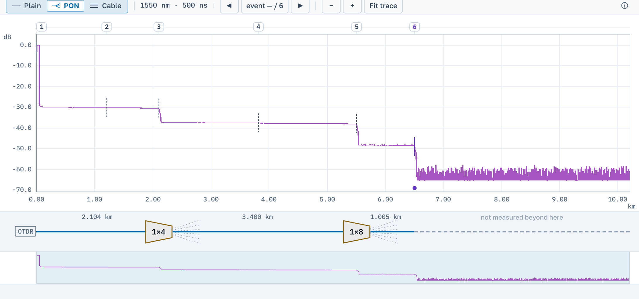
What we do not have: threshold values, a verdict on whether a network passes, any knowledge of PON topology, or any way to say which subscriber a branch belongs to. The loss budget is set by the class of the system in the design, comes from the site documentation, and is not supplied by us in any form.
What the view does not do: it does not hunt for splitters, does not know the topology and supplies no norms. The limit for the excess over the division is one you write into the limits panel, like every other. Past a splitter our own end of fibre gives way to "not measured beyond here": behind a splitter we cannot tell a break from the noise floor, and silence is truer than a guess. The mark reaches the report too: the sheet grows a splitter column and an "over division" one, and a line under the table saying the ratio was declared by you, not measured by the instrument.
Next
A PON can also be measured while it carries service: instruments have a separate port at a wavelength the subscriber's filter blocks, and the working channels are left untouched. That is usually 1625 or 1650 nm, and vendor PON acceptance procedures are written around them. In the file such a trace differs from an ordinary one only by the wavelength in its header, which is the only mark saying the network was live when it was measured.