Examples
What an OTDR trace looks like
If you have only heard about OTDR traces, looking at one beats reading about it. A ready trace opens below: the curve, the event table, and the cursors people measure a span with. Nothing to install, and no file of your own needed.
The example is drawn by us after real measurements, not taken from somebody's customer. We show nobody our own files, and nobody else's either.
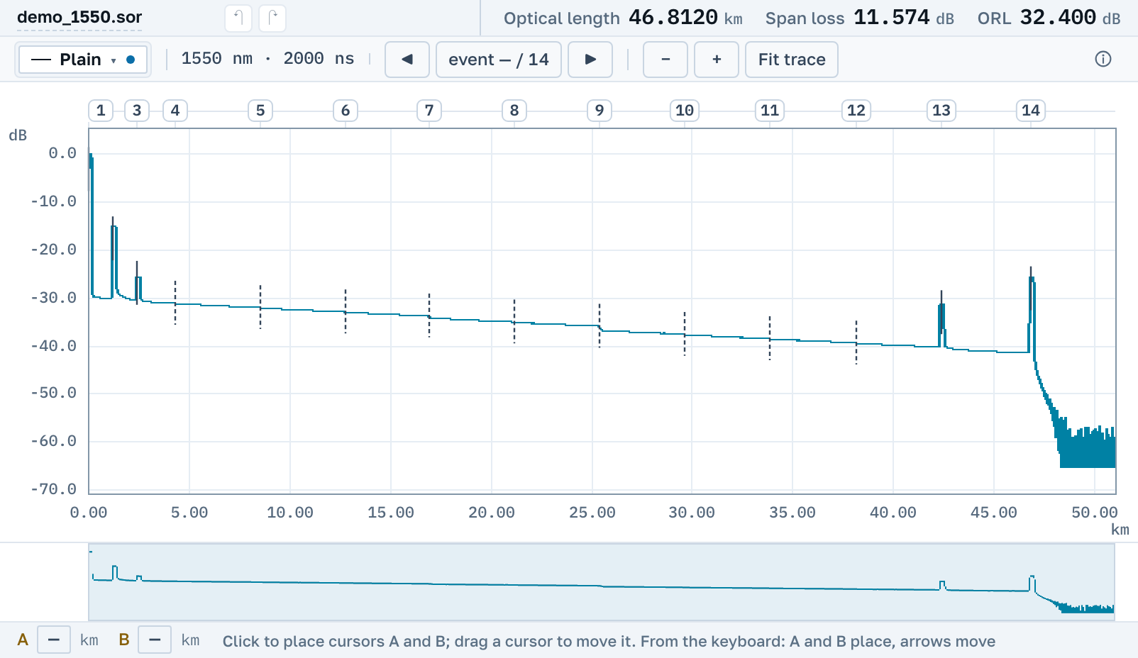
What you can see on this curve
Distance runs left to right, and the level of returning light runs bottom to top. Fibre always draws as a line sloping down: the further along, the less comes back.
A step down
The curve drops for an instant and carries on at the same slope. That is usually a splice: some light was lost and none of it came back. The height of the step is the loss at that joint.
A spike up
A narrow peak with the curve continuing lower afterwards. This is a connector or a mechanical joint: part of the light returned to the instrument. Behind the peak lies a blind stretch where a small event cannot be seen at all.
A drop into noise
The curve falls and then trembles near the bottom. That is the end of the fibre, either its face or a break. One trace does not always tell those two apart, and the instrument hedges at that point as well.
Four examples, all different
The first one opens with the button above. The rest sit inside, on the shelf: the application opens them itself and points out what to look at.
A long span at 1550 nm
Almost 47 kilometres with joints along it and one splice clearly worse than its neighbours. It is the file to start from: cursors, the three ways of computing loss and the acceptance thresholds are all shown on it.
The same line at 1310 nm
The same fibre shot at the other wavelength. Put both curves on one graph and you can see that a bend loses differently at 1310 and at 1550, while a splice loses about the same. That is how the two are told apart.
The reverse shot, B to A
The same line from the other end. A one-way measurement of a splice is always wrong in one direction, and on a facing pair you can watch it happen: the loss of one joint differs between the two ends, and the average is what people take as true.
A PON network with splitters
A cascade of two splitters, 1×4 followed by 1×8. Their steps are deep, and the question here is a different one: how much the splitter took by its own rating, and how much it took on top of that.
An opened example stays in your browser's file list until you remove it with the cross. It does not travel to us: we have it already.
Your own file opens the same way
If you already have a file, you do not need the examples: drop it into the window. Both generations of .sor are read, along with .trc from three different instruments, .msor, .bdr, .csor, .tst and other formats, an archive included. What the file is we work out from the bytes, not from the extension.
No account, no install, and the operating system does not matter. An opened trace can be handed on by link to somebody who has nothing but a browser.