Knowledge base · What is this on my trace
The splice that seems to gain: where the minus comes from and why the reverse shot fixes it
A splice cannot add light, and yet an OTDR sometimes reports a negative loss at one. The instrument is fine and the splicing was done right: this is what a joint between two fibres of differing backscatter coefficient looks like.
The minus also tells you something about the whole fibre: if one joint reads off in one direction, then every other joint on that fibre is measured off too, merely not far enough to flip the sign.
By Ilya (engineer, 6 years in fibre optics) ·
On this page
What it looks like on a real trace
Below is a demonstration trace that ships with EXFO software, opened in our viewer: three splices about ten kilometres apart at 1310 nm. At two of them the curve steps up, and the table prints their loss as −0.305 dB and −0.205 dB.
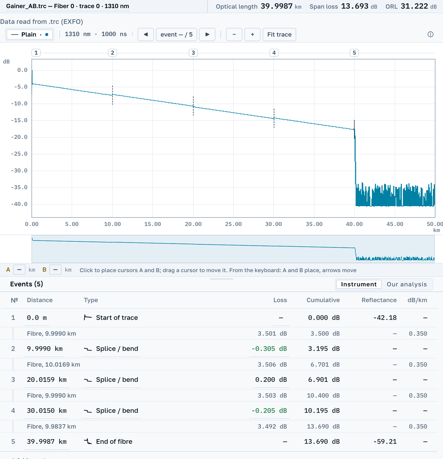
Nothing in the line can add light, so each of these numbers is a loss plus an error with a sign.
What the OTDR actually measures
The splice itself is invisible to it; what it sees is the level of light the fibre sends back, before the joint and after it.
Backscatter is a property of the fibre
How much light a fibre returns to the instrument depends on the fibre itself: its core, its aperture, its batch. Two lengths off different drums return different amounts even across a perfect splice.
The instrument takes a difference of levels
Joint loss is the difference between the level before and the level after. If the fibre past the joint returns more than the fibre before it, the difference comes out the other way, and the trace shows a step up. No energy was added: what changed is the share that came back.
The error changes sign with the direction
Connect from the other end and the same backscatter mismatch enters the measurement with the opposite sign. That is why a joint is measured from both ends and the mean taken: the mismatch cancels and the real loss of the joint is left.
Why the mean, and why exactly the mean
Write the true loss of the joint as S and the backscatter mismatch of the two fibres as ΔK. From one end the instrument reads S + ΔK; from the other, S − ΔK. Add the two and halve them, and ΔK is gone: S remains. The cancellation is exact, with no approximation in it, provided both measurements are of the same joint.
A one-way figure is incomplete even where no minus appears. At every joint it is overstated at one end by exactly as much as it is understated at the other. The minus shows up where ΔK grew larger than the loss and turned the sign over.
This is why acceptance testing checks splices from both ends even when the total link loss passes. A one-way measurement answers "what does it cost to traverse the link this way"; a two-way one answers "what is this splice".
What to do about it
- Do not accept or reject the splice on this number. The one-way loss of a joint between different fibres is wrong in both directions: too low from one end, too high from the other.
- Measure the same fibre from the far end, at the same wavelength.
- Take the mean of the two readings for each splice. The backscatter error enters them with opposite signs and cancels.
- If only one end can be reached, say so in the report and judge the link by its total loss: over the whole line the error of one joint hardly shows.
How to do it here
Open both traces, the forward one and the reverse, in the workspace and press Choose the reverse trace. Separate .sor files do not record the direction, so which of the two is the reverse is for you to say. What follows is a joint table where every joint carries its own figure, the reverse figure, and the mean of the two.
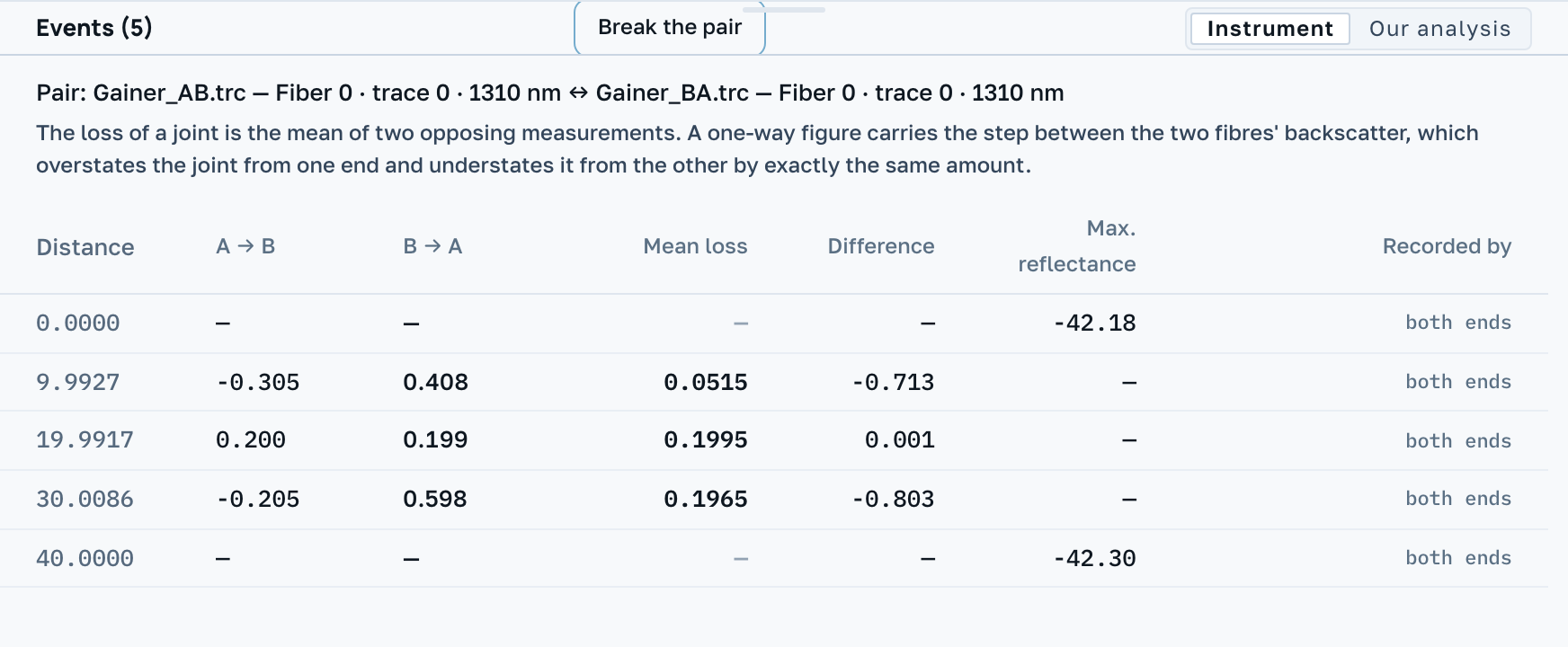
On this pair both gainers turn out to be ordinary splices: −0.305 dB one way and 0.408 dB the other give a mean of 0.0515 dB, and −0.205 with 0.598 give 0.1965 dB. The third splice reads 0.2 dB from both ends, which is what a joint of two matching fibres looks like.
Apart from the table, the reverse curve can be laid on the chart with Reverse trace: it is drawn mirrored, so its metres read from the far end, and aligned at cursor A. The size of that alignment is written in the legend; without it, a level could be read off the curve that does not exist.
We also check what stands in the way of pairing: if the two sides were computed with different indices of refraction, their distances live in different systems, and we say so before you start matching closure numbers. The same for a differing backscatter coefficient: that mismatch is precisely what the mean removes. And where the instrument recorded no loss on one of the sides, there is no mean at all, because half of one side is not an average but the same one-way figure halved.
With a single trace the table keeps the minus and shows no mean, because we do not guess the reverse reading. The program does not decide whether the splice passes either. You set the threshold.
An event only one end recorded
A joint can be in the table of one end and absent from the table of the other. Below is a pair from the EXFO sample set, one fibre measured from both ends at 1310 nm through a launch cable at each end. From end B the splice at 5.67 km reads 0.153 dB. The instrument at end A wrote no row there.
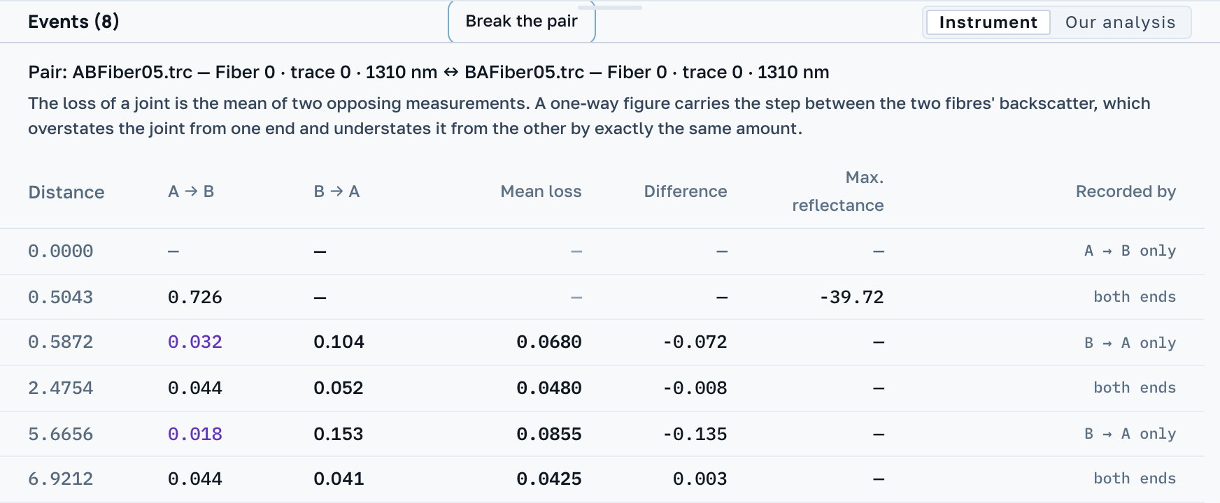
The column Recorded by says which end wrote the row. For the missing half we measure the same place on the other curve, here 0.018 dB, and print it in our own colour. The mean of the two is 0.0855 dB. It is the case from the first section again: the backscatter mismatch added to the loss from one end and took away from it at the other.
Next
Averaging cures only a backscatter mismatch. Different acquisition settings, different pulse widths or different indices of refraction on the two sides produce a discrepancy the mean will hide but not remove.