Manual
How to use OTDR Master
Nineteen sections about the application itself: what to press, what the answer on the screen means, and what signing in by email and the Professional plan give you. The physics of the measurement is covered separately, in the knowledge base.
On pulse width, dead zones, event types and loss budget: knowledge base
1 Open a file
Drop a file anywhere in the window or press Open file. No file at hand? Open an example puts a real 46 km trace on the screen, and everything described below works on it.
It is not only .sor. Instrument formats from EXFO, Anritsu, Fluke, Yokogawa and others open the same way, and a .zip, .7z or .rar archive needs no unpacking: the application reads the traces straight out of it and asks which ones to open.
Another vendor's format opens, but does not edit
A file written in anything other than Bellcore opens read-only: it cannot be edited and cannot be saved back. When you do need to work on it, press Convert to .sor. A second row appears in the list, an editable copy.
The file you open travels to our server and is parsed there; nothing is read in the browser. What we do with it is in the terms of use.
The list of open files is on the left. Clicking a card makes that file the working one: its figures move into the table and the parameters. The eye keeps a curve on the chart without making the file the working one, and the cross removes the file altogether. The number on the left of a card is the file's place in the list. Remove a file and the numbers below it move up, with no gaps.
2 Look at the trace
The mouse wheel changes the scale, dragging across the chart zooms into the piece you outlined, and a double click brings back the whole trace. So does Fit trace, while Fit all curves picks a window where every open curve fits.
Below the chart is the overview strip: the whole trace with a rectangle around the visible piece. Drag it with the mouse, click past it to move the window there, or roll the wheel to travel along. It never changes the scale; the zoom buttons do that.
The decibel scale follows whatever is on the screen. Zoom in on a splice and the vertical stretches by itself, so a step invisible across the whole trace becomes plain.
Notes on events
Every event the instrument recorded carries a short note above the curve: the type, the loss, the fibre attenuation after it. If they are in the way, Hide hints in the panel above the chart takes them off, and the choice is remembered for next time.
Stack curves spreads them out vertically so you can see the shape of each. While they are stacked no level can be read off the axis for any of them, and the application says so right under the chart.
3 Measure with the cursors
Click the curve twice: cursors A and B appear. A cursor can be dragged, and from the keyboard the A and B keys place them while the arrows move them. The strip under the chart prints the distance and level at each, the length of the span between them, and three measurements.
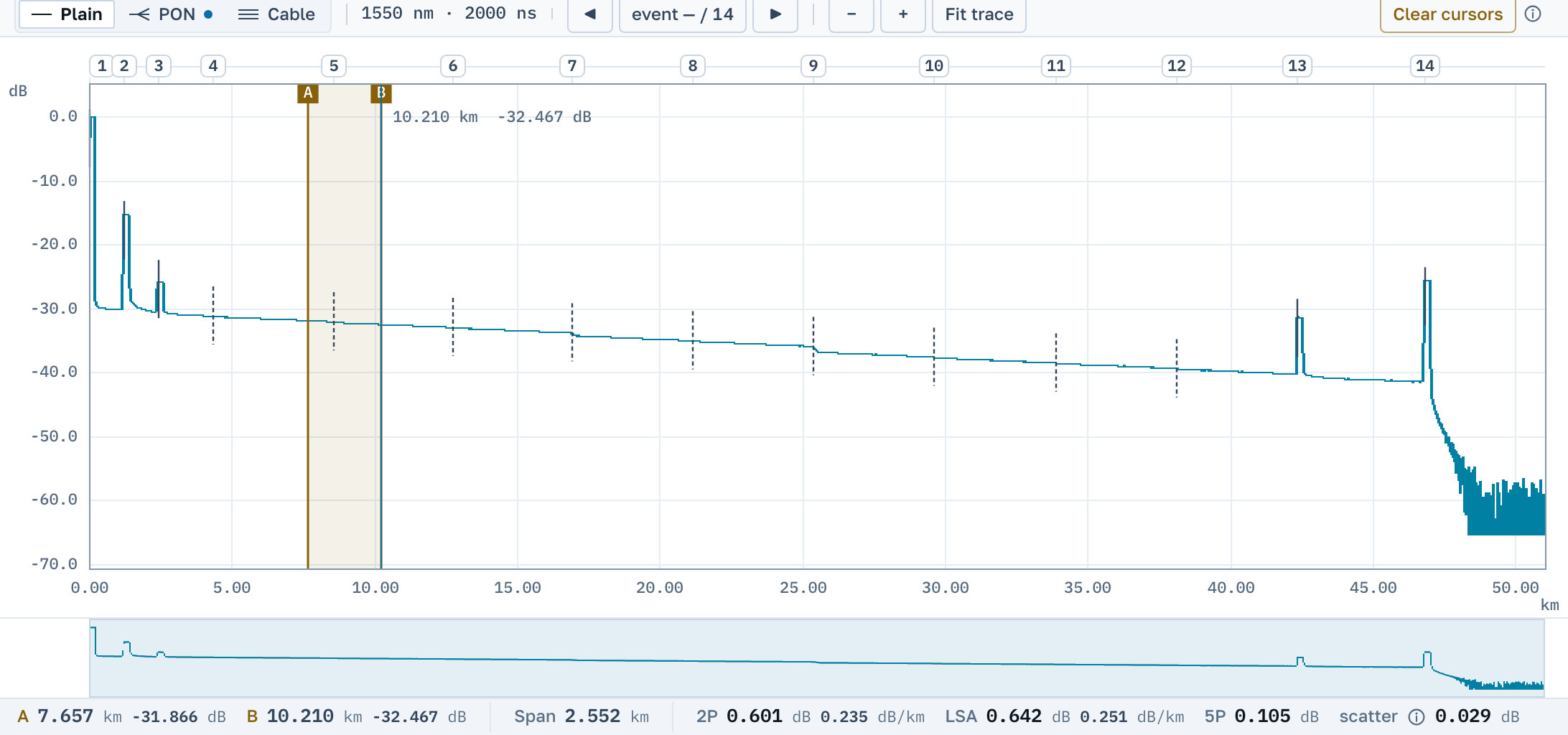
Three figures answering three questions
- 2P is the level difference exactly under the cursors. It is always there, it assumes nothing, and it is the figure that goes into the acceptance sheet for a span.
- LSA is least squares between the cursors. On a noisy fibre it is steadier than 2P.
- 5P is the loss of the splice itself: two lines are fitted to the clean fibre outside the cursors, and the figure is the gap between their continuations.
Read 5P. With 2P there is fibre left between the cursors, and its attenuation is added to the loss of the event.
It means there is no figure here worth trusting: too little clean fibre nearby, or the fitted lines came out ragged. Their scatter is printed next to the dash, and in that spot the measurement to use is 2P.
To take the cursors off, press Clear cursors in the same panel above the chart.
4 The event table
The rows your instrument wrote are at the bottom left: number, distance, event type, loss, reflectance and the loss accumulated from the start of the trace. Clicking a row aims the chart at that spot, so there is no hunting for the event by hand.
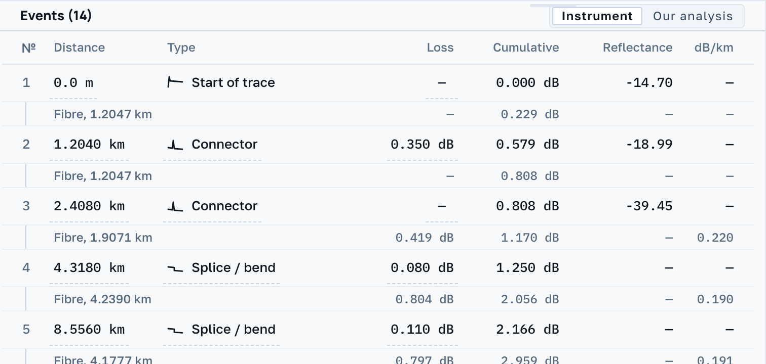
A row can be corrected: Edit the figures changes the values, Delete event removes the row, Add to the file creates a new one. These are edits to the file, and they can be undone.
The instrument or our analysis
The Instrument / Our analysis switch changes the question the table answers. On the left is what the file says. On the right is what we found walking the curve with our own detector, and our rows carry a dot.
A lit switch means we have something to add: either the instrument wrote no rows at all, or it ended the fibre where the curve carries on.
That is your instrument's detection threshold, recorded in the file at capture time: an event quieter than the threshold never enters the table. Nothing is lost and nothing is broken on our side. It is a setting of that measurement.
5 Acceptance thresholds
The Limits tab is on the right. Type in what your contract asks for: splice loss, connector reflectance, fibre attenuation, total span loss. An empty field is not checked at all.
As soon as a threshold is set, a verdict column appears in the table, a breach turns red and says in words how much was measured against which threshold. The summary for the whole file sits next to the table.
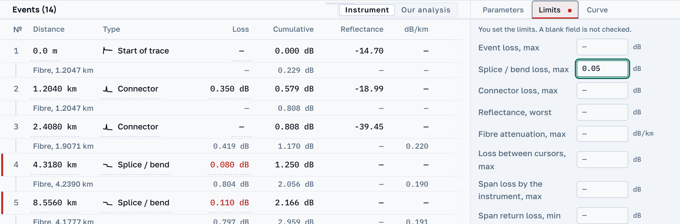
If the file carries the instrument's own thresholds, the application says so and offers Use these. That is your choice to make, not our default.
There is not a single ready-made set of values in the application, industry or "typical". The norm comes from the contract, and it is typed in by whoever signs the work off under that contract.
A quantity the instrument never recorded is not judged: instead of a green "within limits" the row says plainly that there was nothing to check.
6 Compare fibres
Open a whole drum at once: a folder, a handful of files or an archive. The chart takes as many curves as fit, each in its own colour, and the colour belongs to the file, so removing a neighbouring curve repaints nothing.
Curves beyond the eighth are drawn in a muted shared tone: there are exactly eight distinguishable colours, and a ninth shade would make the comparison a lie. The working curve is always drawn on top.
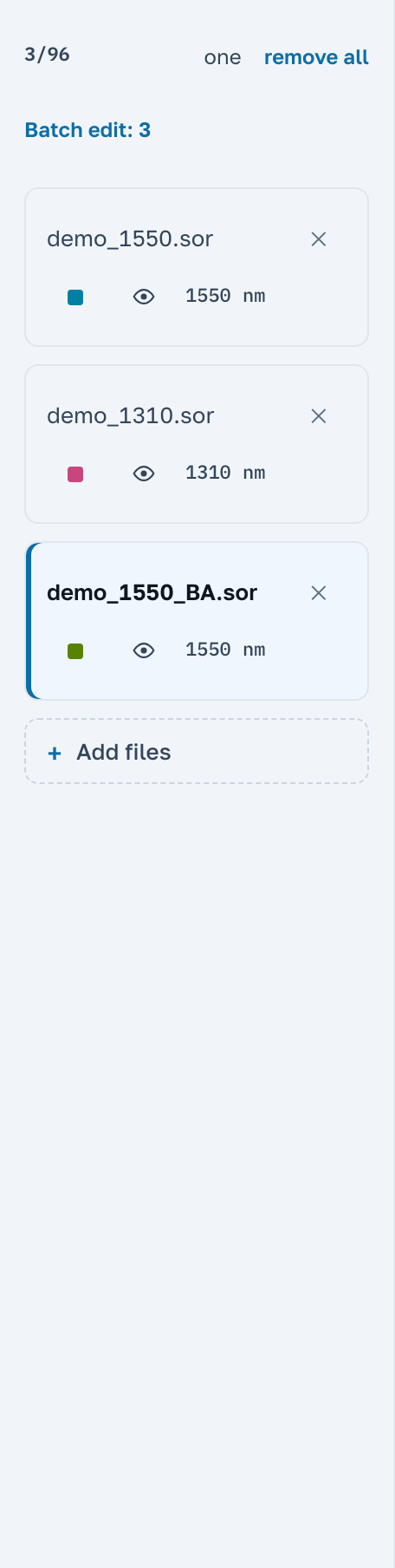
Leafing through fibres one by one
one in the list header leaves only the working curve on the chart, and from then on clicking a card replaces it instead of adding to it. That is how you go through forty-eight fibres in a row. all brings back exactly the set you had before. You can leaf through from the keyboard too: click a card, and each press of the up or down arrow opens the next file. Home and End open the first and the last.
From the ninth file onwards a search box appears above the list. It looks through the name, the path inside an archive and the instrument's wavelength, so 1310 finds a trace whose name does not carry that number. Type a file number with a sign: #7 leaves the seventh file in the list, and Enter opens it. Without the sign, the number is looked for in the names.
7 A pair of opposite directions
A one-way measurement of a splice always lies a little: the fibres on either side of the joint scatter light differently, and at one end the loss is overstated by exactly as much as it is understated at the other. The truth is the mean of the two opposite measurements.
Open both traces of one fibre and press Choose the reverse trace. The application matches the events by distance and shows the pair table: forward, reverse, mean loss and the spread between them. Break the pair puts everything back.
The reverse curve is drawn mirrored (Reverse trace), and the application picks the offset itself so that the cross is readable.
That is a gainer: not an instrument error and not a defect, but the same difference in backscatter seen from one side. The mean over the pair puts the figure back where it belongs.
8 PON networks
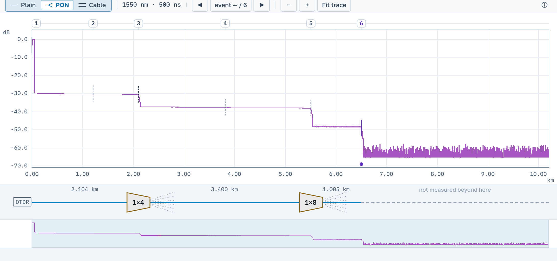
PON view is turned on by the Plain / PON / Cable view switch above the table. Turned off, it changes nothing whatsoever in the file or on the screen.
We do not decide the event type for you: you name the splitter ratio yourself, choosing it in the event row. After that the application works out the power division and shows how much the event lost on top of it. That excess is what the conversation with the installer is about.
Where a step looks like a splitter, a suggestion appears; Mark in the row accepts it, and the button in the table header accepts every suggestion at once. The same row takes the mark off again.
In this view a span diagram is drawn above the chart: the instrument, the sections with their lengths, the marked splitters and a dashed line where the analysis stops.
9 Edits and undo
The measurement header is edited on the Parameters tab: cable, fibre, points A and B, operator, index of refraction. Click a value to open the field, Enter saves, Esc cancels.
The index of refraction changes the length: the previous value appears under the field, together with how the optical length and the end of fibre moved. The file name is edited where it is written, in the line above the chart, and it travels into the share link and onto the report sheet.
Editing the curve
Crop cuts the trace at the cursors or at the visible piece, Level shift moves it as a whole, Repair one sample fixes a single spike. Each edit says in advance exactly what it will do.
Everything can be undone: with the buttons above the file name or with Cmd/Ctrl+Z, while Cmd/Ctrl+Shift+Z brings the edit back. Next to them is a counter of how many edits this file already carries.
10 The report and the link
The Report button builds a sheet for the fibre: the job header, the curve, the event table, the totals and, if thresholds are set, the verdict. The sheet is shown in full before you download it, so you can look it over and choose what to include. The first row of the window, Sheet language, prints the sheet in a language other than the screen's, for a customer abroad, say. The choice is remembered in this browser.
Download PDF gives you the sheet. Download CSV gives the same events as a table for Excel, and it opens once you have signed in by email.
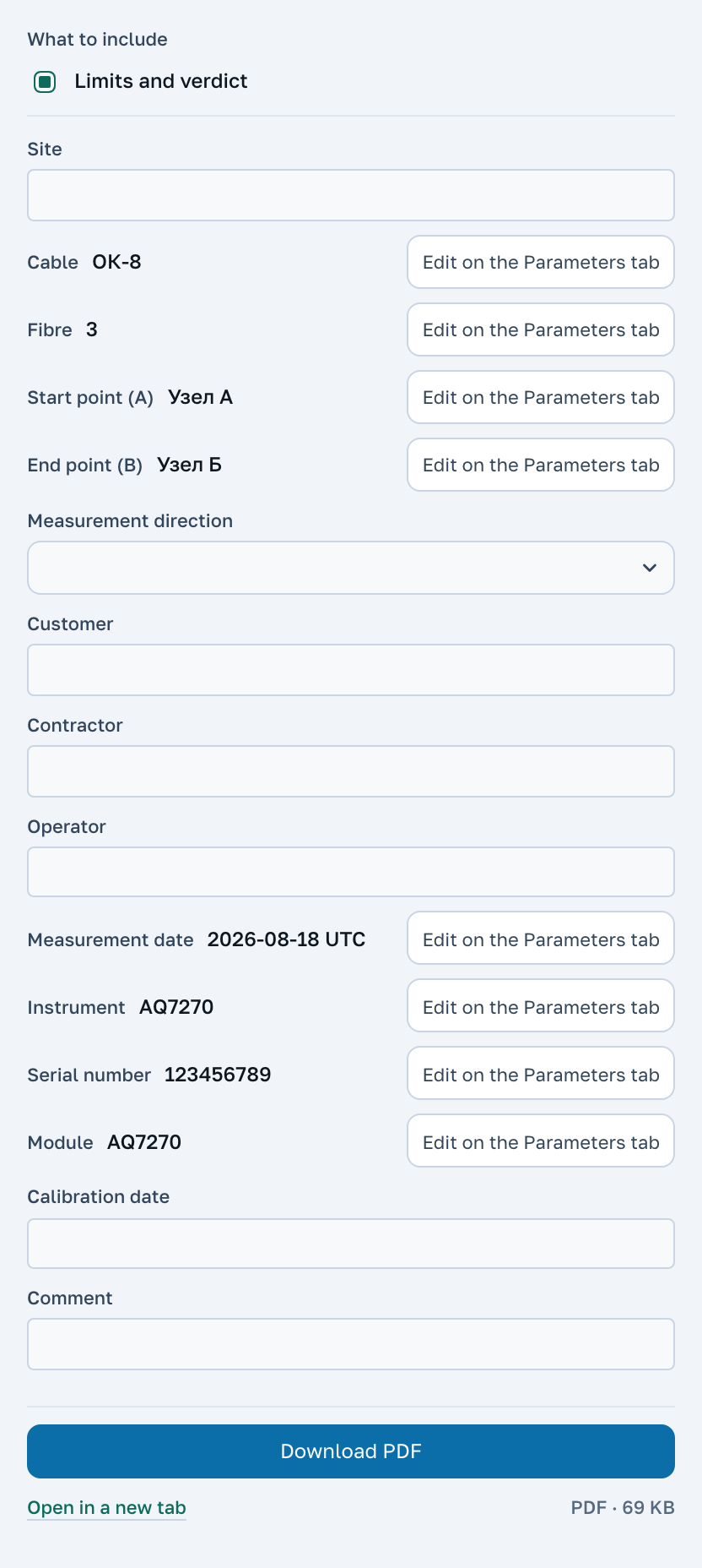
The sheet carries a code and a square for a phone camera. With them your customer opens the same trace at our place and looks at it without installing anything.
Sharing a trace
Share makes a link that lives two weeks and puts it on the clipboard. It opens a copy: the person you sent it to works on it like their own file, and their edits never touch your screen.
11 Gestures and keys
Everything done by hand, in one table.
| Action | What happens |
|---|---|
| Mouse wheel | Scale along the distance axis |
| Drag across the chart | Zoom into the outlined span |
| Double click | Back to the whole trace |
| Click on the curve | Place cursor A, the next click places B |
| The A and B keys | Place a cursor from the keyboard |
| Left and right arrows | Move the selected cursor |
| Click on an event row | Aim the chart at that event |
| Cmd/Ctrl+Z | Undo an edit to the file |
| Cmd/Ctrl+Shift+Z and Cmd/Ctrl+Y | Redo what was undone |
| One finger on the chart | Travel along the fibre |
| Two fingers | Scale on a phone or tablet |
| Tap the curve | Place a cursor, the next tap places the second |
| Up and down arrows in the file list | Open the neighbouring file |
| Home and End in the file list | Open the first or the last file |
There is no drag-zoom and no double click on a phone: two fingers and the Fit trace button do that work instead.
12 Why the figures differ from your instrument
A difference of hundredths of a decibel is ordinary, and it does not mean anyone made a mistake. Below are four reasons the figures legitimately disagree.
- The method. 2P, LSA and 5P count the same splice differently, and the instrument used its own method for its own table. Compare like with like.
- The length. There are three: how far the recording went, the distance between the operator's markers, and the end of the fibre itself. Attenuation per kilometre worked out over different lengths differs several times over.
- Optical return loss. Vendors compute ORL under different conventions: with or without the reflection from the far end, from the start of the span or from zero. We show what the file records.
- The detection threshold. The rows in the table were chosen by the instrument at capture time. Our detector does not inherit its threshold, which is why "Our analysis" often holds more rows.
What we never do is write on the instrument's behalf. A field the file does not carry stays empty instead of turning into a zero.
13 How many files and how large
One file up to 3 MB. That is generous: the heaviest trace we have ever seen is eight times smaller. The same allowance applies to each entry inside an archive.
Without signing in the workspace holds 96 files and the chart holds 8 curves at once. Signing in by email raises those to 576 and 24. The files live in your browser and survive closing the tab.
An archive is unpacked up to 32 MB of content. Whatever did not fit is named one by one with the reason, rather than dropped in silence.
14 Three plans
Looking, measuring, editing and handing over one fibre at a time is free, and it will stay that way. Signing in by email is free too and adds room, a cabinet and a report that links back to the trace. Professional is paid: it is for jobs with dozens of fibres that go to the customer as one document.
| What you do | Not signed in | Master | Professional |
|---|---|---|---|
Open a file from any instrument, measure, edit, save as .sor | yes | yes | yes |
| PON mode, a link to the trace for a colleague | yes | yes | yes |
| A PDF report for one fibre | yes | yes | yes |
| Traces in the workspace and curves on the chart | 96 · 8 | 576 · 24 | 2048 · 48 |
| Room for files in the browser | 32 MB | 128 MB | 512 MB |
| Your work from any computer, “My cabinet” | no | yes | yes |
| Code and QR on the report, CSV export | no | yes | yes |
| A report on a fibre from both ends, with the average of the pair | no | yes | yes |
| Projects | no | one, editable for 3 days | unlimited, always editable |
| Cable summary: the whole set as one PDF and one Excel workbook | no | no | yes |
| Batch edit: a header field in every file at once | no | no | yes |
| Cable mode: checking fibres against the drum's factory data | no | no | yes |
| Whole project: completeness, reverse traces, the project report | no | no | yes |
Count how many reports you made one by one for your last job. If there were more than ten fibres, the cable summary builds them in one pass and batch edit spares you the same edit in every file. You can try it free for three days: see “Trial” below.
15 Master: signing in by email
Press Sign in in the header and enter your address. A letter arrives with a link and a code: open the link or type the code into the same window. There is no password. The link in the letter works for 15 minutes and only once.
Files you opened in this browser before signing in move to your account. From then on your work is visible from any computer and from your phone: open a trace on the laptop, and at home it is already in the list.
What signing in adds
- More room. 576 traces in the workspace instead of 96, 24 curves on the chart instead of 8, and 128 MB in the browser instead of 32.
- Code and QR on the report. Your customer points a phone camera at the square or types the short code and sees the same trace at our place, with nothing to install. The link on the report does not expire until you remove it.
- CSV. The numbers from the report as a table, for your own test record form.
- A report on traces from both ends. A fibre measured from both ends on one report, with the average of the pair. It covers one fibre; a whole set of fibres is what the Professional cable summary does.
- One project. See “Projects”.
My cabinet
Opens from the menu under your address. Files are on the left, reports on the right, both laid out by day; the calendar marks the days with work with a dot. Search finds a file by name and a report by name or by the code printed on it.
Every report has Download again, which gives you the same file you handed over. Delete removes its link, and the code on paper stops opening the trace. The counters at the top show how many files you opened, how many reports and links you made, how many times your customers opened your reports and when they last did.
16 Projects
A project holds one job: a line, a cable or an order. It has a name, a customer, ends A and B and a description. The job's files and reports live in it together, and six months later you find it in the cabinet by customer, file name or report code.
Press Projects above the file list, then New project. The tick in the window puts every file in the list into the project at once; clear it if not all the files are there yet. After Create project a strip with its name appears above the list.
While a project is open
- The list shows exactly the project's files.
- A file dropped into the window goes into the project.
- The cross on a card takes the file out of the project, and Put back in the notice returns it. The file itself stays in the cabinet.
- A report made while the project is open belongs to it, and the cabinet names the project next to the report.
- The project name in the strip opens its card, where you edit the fields and find Mark as handed over. Close brings back the ordinary list.
Master has one project
On the free plan there is one project, and it can be changed for three days from the moment you create it; the strip says how many days are left. After that it is closed for edits: nothing can be added to it or taken out of it, and its files cannot be edited anywhere, not even when opened from the ordinary list. It cannot be deleted to make room for a new one either.
A closed project can always be read. To fix one of its files, open the file and press Open separately: a copy appears outside the project, and you can do anything with it. The job you handed over stays exactly as you handed it over. A link or a report code pointing at such a file opens a copy too.
Professional has as many projects as you need, they are always editable, and Delete project on the card removes a project while its files and reports stay in the cabinet. Once you pay, closed projects open for edits again.
17 Professional: what you pay for
Professional takes over what you otherwise repeat by hand on every fibre: report after report, and the same edit in every file.
Cable summary
Open all the files of the cable, press Report and choose the “Cable” line with the file count under “What to include”. The server works out the fibre number and the end of every file itself: from the file, from its name or by order. The result is the “Fibres and ends” table: correct it where the server got it wrong, and mark a spare file leave out.
- The “Cable fibres” sheet. A row per fibre: length, end-to-end loss from each end and the average, attenuation, average splice loss, ORL, the worst event with its distance, and a result against your thresholds. Average, minimum and maximum for the cable underneath.
- The “Splice losses” sheet. The places where most fibres have an event, and each fibre's splice loss at each place, averaged over the two ends.
- The “Fibres and their files” sheet. Which file went into which row, and what the application noticed about each pair.
- A sheet for every fibre if you tick A sheet for each fibre: the same report as for one fibre, all in one PDF.
Download PDF gives the summary as one document, Download Excel gives it as a workbook with a sheet per wavelength. Compare wavelengths adds a sheet with splice losses at two wavelengths and the difference between them. One summary takes the whole workspace, up to 2048 files, and the fibre sheets come in the same PDF. A set of more than 96 files has no preview: it is built when you press Download PDF, the window shows how far the build has got, and it takes a few minutes.
Batch edit
The instrument got the date wrong, the cable field holds a factory name, and the test record needs the job name? The batch edit button above the list opens a window: pick a field, type the value, and it goes into every file visible in the list. You can take several fields: cable, fibre, points A and B, date, operator, index of refraction, wavelength and other header fields.
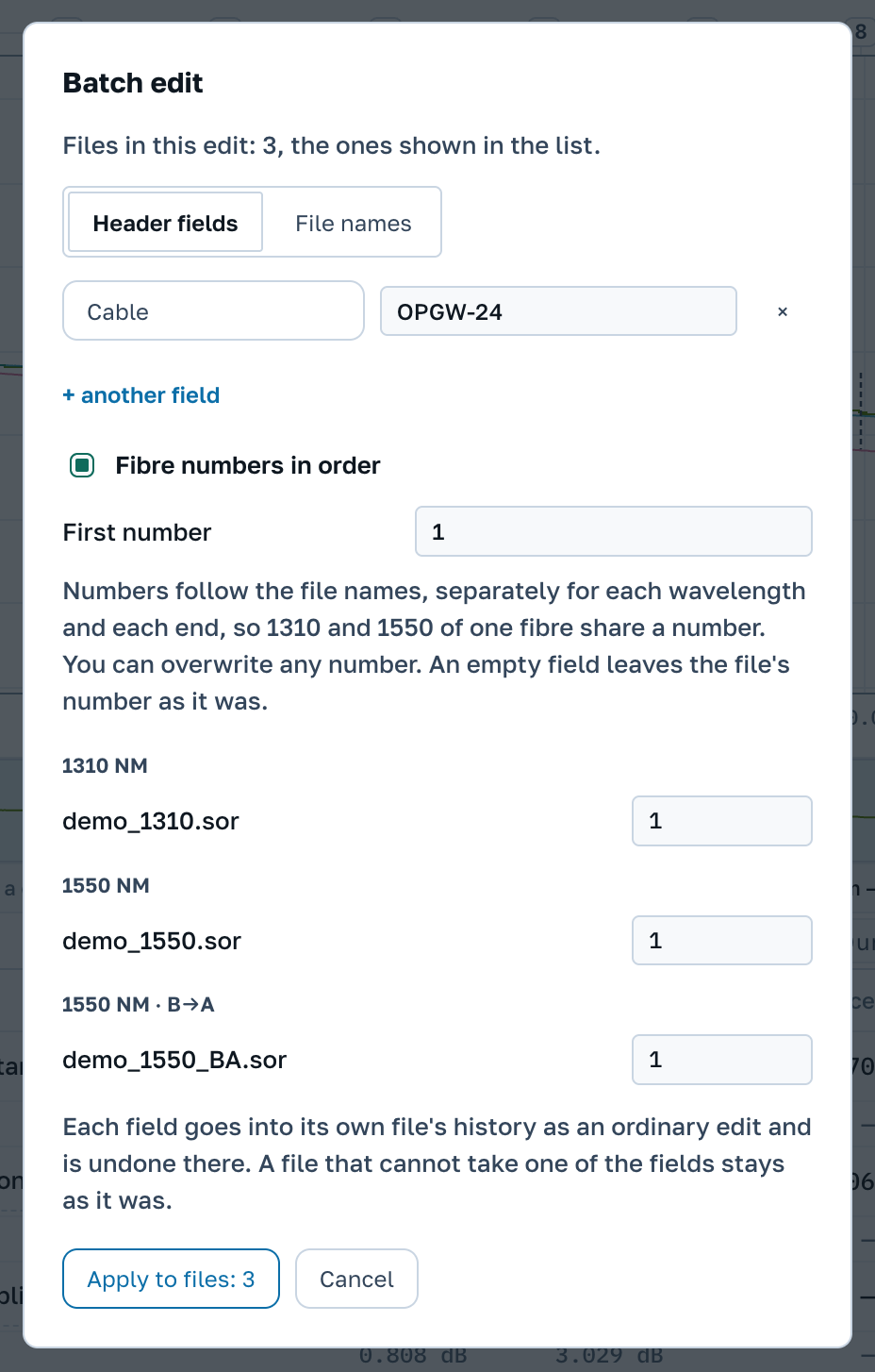
Each value goes into its file's journal as an ordinary edit and can be undone there. A file the field does not fit stays as it was, and the window names it.
The Fibre numbers in order box writes a fibre number into each file’s header. Numbers follow the file names, separately for each wavelength and each end, so 1310 and 1550 of one fibre share a number. First number sets where to start, and any number in the list can be overwritten by hand.
The File names tab renames files by a pattern. Buttons put each file’s name, cable, fibre, wavelength and end into the pattern, and {fibre:3} pads the number with zeros to three digits. Any name in the list can be corrected by hand, and the window marks names that coincide.
Cable mode
Incoming inspection of a drum: enter the factory data once, and every fibre is checked against it for length, attenuation and index of refraction. Anything beyond your tolerance turns red, and the line above the chart gets the label Outside factory data.
How to enter the factory data and what each cell means is on a separate knowledge base page.
More room and projects
2048 traces in the workspace, 48 curves on the chart and 512 MB in the browser. As many projects as you need, and they do not close for edits while you are paid up.
The whole project
The bar of an open project has two buttons. Completeness opens a grid: a row per fibre, a column per wavelength and end. An empty cell means that end was not measured at that wavelength.
Under the grid is the “File layout” list: every file with its fibre number and end. If the file names are mixed up or the instrument wrote the wrong thing, type the right ones in the file’s row. Number them in the “Number in a row” line numbers the files of one end in the order of their names, for each wavelength separately. The change is kept in the project and applies to the grid, the reverse traces and the report.
In a project the reverse trace pairs up by itself, by fibre number and end. Where there is no pair, the line above the events table says why: there is no reverse trace, the file has no fibre number, that end is already in another file, or the reverse trace was taken at another wavelength. A pair you name with Choose the reverse trace is written into the project.
Project report opens the report window on every file of the project at once, including files that are not open in this browser. Download PDF and Download Excel give the summary for the whole project. PDF for every file makes a PDF report for each fibre of the project without opening the files: both wavelengths and both ends of a fibre go into one report, and each report is put into the project at once with its own code. Download all (.zip) gives the project as one archive: the originals folder holds the files as they were added, sor holds each of them as .sor with its edit log, and reports holds the reports, Excel workbooks and CSV tables made in the project plus a fresh summary of the whole project.
Your own sheet
Report templates live in your account page, in the «Report templates» row; Set up templates in the report window leads there too. On the left is the sheet for the open trace, on the right the settings: a logo, up to four lines of company details under it, the sheet title and the header fields. A field can be switched off, renamed, moved up or down, or you can add your own with its own value. Below that you choose what the sheet prints and the signature lines at the end. Edits save themselves, and the sheet on the left changes with them.

You can have up to ten templates. The one marked Print by default prints until you pick another in the Report template row of the report window. In the project card you tick the templates the project prints with: the archive and PDF for every file come out in each of them, one folder per template. Editing a template changes the next reports; the ones already issued stay as they were.
If even your own sheet does not fit, the numbers go to Excel. Download Excel in the project report gives a workbook with the project summary, one row per fibre, and with A sheet for each fibre ticked the same workbook gets the event table of every fibre. From there you build the test record in whatever form the customer asks for.
18 Trial
Wherever the application says something is part of the paid plan, Try it free sits next to it: at the cable summary, at batch edit, in cable mode and in the second project window. Pressing it turns on the whole of Professional for three days, with no limit on reports. Each account gets it once, and you need to be signed in.
The menu under your address says the date the trial runs to.
Projects during the trial
- The trial gives two projects in all, counting the one you already had as a Master.
- A new project can be changed until the trial ends; the window that creates it names the date.
- Projects cannot be deleted during the trial.
- A Master project whose three days are over stays closed for edits: the trial does not reopen it.
When the trial ends, the paid features close, and the trial's projects close for edits the same way a Master project does. Your files, reports and projects stay with you.
19 Payment
Buy Professional is in the menu under your address and next to every “paid” notice. There are two periods: a month of 31 days for $14.97 and a year of 365 days for $119.88. What you get is the same.
Payment is in dollar stablecoins: USDT on TRON or USDC on Base. On the payment page pick the period and the method and press the invoice button, which shows the amount. The page then shows the address, a QR code for your wallet and the amount to the last digit: that amount is how we recognise your payment, so send it exactly and add the exchange fee on top.
An invoice is valid for a day. You can close the page: access opens by itself as soon as the transfer arrives, and a payment confirmation comes by email. The days left are shown in your account, on the chip next to your address, together with a checkbox for a reminder 7 days before the end. Nothing is charged automatically. If you pay again before the period ends, the new period is added to what is left.
Can’t pay this way? Choose Card, transfer or invoice: card or transfer, an invoice to a company, or another way. The request comes to our inbox, and we reply within 24 hours.
Next
The manual describes the application. The measurement itself, the instruments and field practice are covered in the knowledge base.